Scaling an Instance Segmentation Dataset with Active Labeling in 3LC¶

How we turned 310 labeled fish into tens of thousands - all in a day’s work.

The DeepFish dataset comprises nearly 40,000 video frames of fish in diverse ocean habitats. Available at the dataset website, it offers labels for classification, localization, and segmentation tasks. While the entire dataset includes fish/no-fish classification labels, the initial segmentation dataset consists of only 620 images, with only half containing fish.

The research paper accompanying the dataset reported a labeling time of 5 minutes per image for segmentation, totaling 25 hours for the initial 310 labeled images. In this article, we demonstrate how we leveraged active labeling in 3LC, starting with these hand-labeled samples, to expand our labeled dataset to over 23,000 images – a more than 37x increase – spending less than a day of work in the 3LC Dashboard. Our model-guided approach accelerated the process while maintaining high label quality, allowing us to train a significantly better model.

[ ]:

Active Labeling Approach¶

We adopted an active labeling strategy to rapidly add high-quality labels to the dataset. The key idea is to train a model on the already labeled data, use 3LC to identify batches of confident model predictions and add them to the dataset. 3LC’s versioning capabilities allowed us to experiment with different approaches and retrain models without requiring code modifications.

In more detail, the following procedure was used:

Create an Instance Segmentation Table: We created a 3LC instance segmentation table from the initial semantic segmentation dataset. This example notebook illustrates how to convert semantic segmentation labels into an instance segmentation table. Then, we set the “sample weight” to 1 for the labeled samples and 0 for all unlabeled images.
Train a YOLO11 Segmentation Model: Next, we trained a model on the samples with weight 1, i.e., on the labeled images. Given the limited number of labeled samples, we trained without a validation set for only a few epochs to prevent overfitting.
Collect and explore predictions: We then collected predictions on all the samples with the trained model and explored these in the 3LC Dashboard. We employed various techniques (detailed below) to identify samples and predictions suitable for addition to the dataset, setting the weight of these newly added samples to 1, so they would be included in the following training round.

We repeated steps 2 and 3 iteratively to expand the labeled dataset exponentially.

Techniques for Efficient Labeling¶

High-Confidence False Positives¶

One effective method for expanding the dataset was to focus on high-confidence model predictions with little to no Intersection over Union (IoU) with existing labeled instances. These “false positives” often correctly identified fish not yet present in the labeled dataset. By carefully increasing the confidence threshold to where we felt assured we were primarily looking at genuine fish instances, we could batch-accept thousands of these predictions into our dataset, assigning them a weight of 1 for inclusion in subsequent training runs.

TODO: movie

Leveraging Image-Level Embeddings¶

The image embeddings generated by the YOLO model proved to be very useful. These embeddings, extracted from the model’s spatial pyramid pooling layer, provided insight into how the model we trained learned to interpret and differentiate the images.

For instance, we observed that the model grouped images based on habitat type.

TODO: movie

Furthermore, when instead coloring by the number of fish labels present, a “fishiness” pattern emerged. Samples located towards the top left of this embedding space have a higher concentration of fish, allowing us to quickly batch-assign samples from the bottom right of each cluster (likely devoid of fish) without labels.

TODO: movie

Low-Confidence Sequences and Manual Quick-Adding¶

In certain habitats, the model generated low-confidence predictions for fish and other features like rocks, bubbles, and seaweed. The ability to quickly review and selectively add predictions became crucial in these scenarios. 3LC enables you to quickly add predictions one by one ( key) or skip to the next prediction ( key). We could rapidly add labels by filtering to unmatched predictions, significantly accelerating the labeling process during focused sessions to around one instance every second.

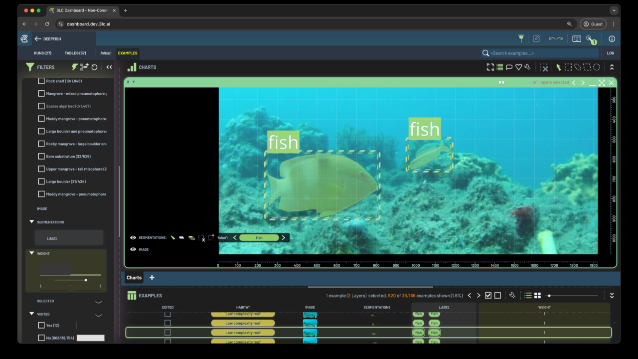
Manual Labeling¶

The initial label set sometimes lacked segmentations for specific fish types, habitats, or other essential features, causing the model to disregard these instances. To address this, we resorted to manual labeling in 3LC. To create a new instance, we add a layer and then use the polygon or brush tools to draw segmentations. The ability to erase (SHIFT key), undo (Ctrl+Z), and redo (Ctrl+X) edits is invaluable for quickly manipulating the labels. Once a few of these fish were added to the dataset, the model started predicting them after the next training run.

Results¶

Through iterative application of these techniques, we successfully labeled over 23,000 images, significantly expanding the DeepFish dataset. While the overall quality is high, some errors inevitably crept in. To quantify the improvement in model performance (the end goal of active labeling), we extracted a representative set of 200 images and carefully verified and corrected their labels. This set included samples from various habitats, with and without fish.

We then conducted two training runs, validating each on the 200-sample test set:

Train on the initial 620 labeled samples.
Train on the current 23,000 labeled samples.

The following results were obtained on the test set:

Initial data: 0.6003 mAP on the test set.
Current data: 0.7863 mAP on the test set.

This represents a substantial improvement in Mean Average Precision (mAP), demonstrating the effectiveness of our active labeling approach.

Challenges and Future Directions¶

While batch accepting predictions significantly accelerates labeling, it also introduces the risk of reinforcing existing model errors. We identified instances where a labeling mistake was added to the dataset, which the model kept making across more images.

To mitigate these issues, we plan to explore the following techniques:

Instance-Level Embeddings: By training a classifier on cropped instance content and randomly selected background crops, we can generate embeddings for every instance. These embeddings will enable us to identify similar objects and confidently batch-delete unwanted labels.
Filtering by Existing Properties: We can leverage existing dataset properties (e.g., segmentation pixel count, location, island count) to filter and remove problematic labels. For example, we identified erroneously added boat segmentations that were large and consistently located in the top right corner of images.

Stay tuned for our next article, where we will delve deeper into these techniques to prune the labels that were added to the dataset – and continue iterating on it – to train an even better model.

References: Saleh, A., Laradji, I. H., Konovalov, D. A., Bradley, M., Vazquez, D., & Sheaves, M. (2020). A realistic fish-habitat dataset to evaluate algorithms for underwater visual analysis. Scientific Reports, 10(1), 14671. https://doi.org/10.1038/s41598-020-71639-x