Semantic Segmentation

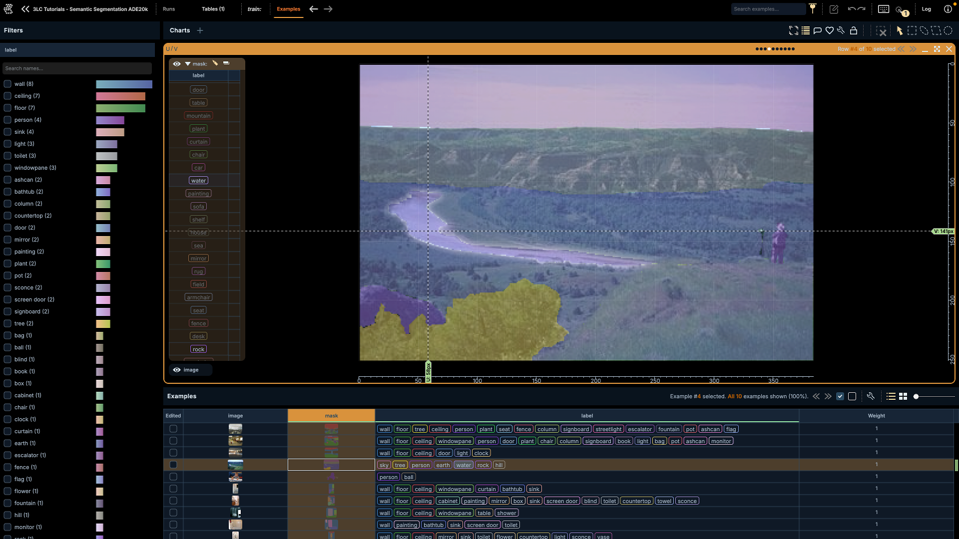
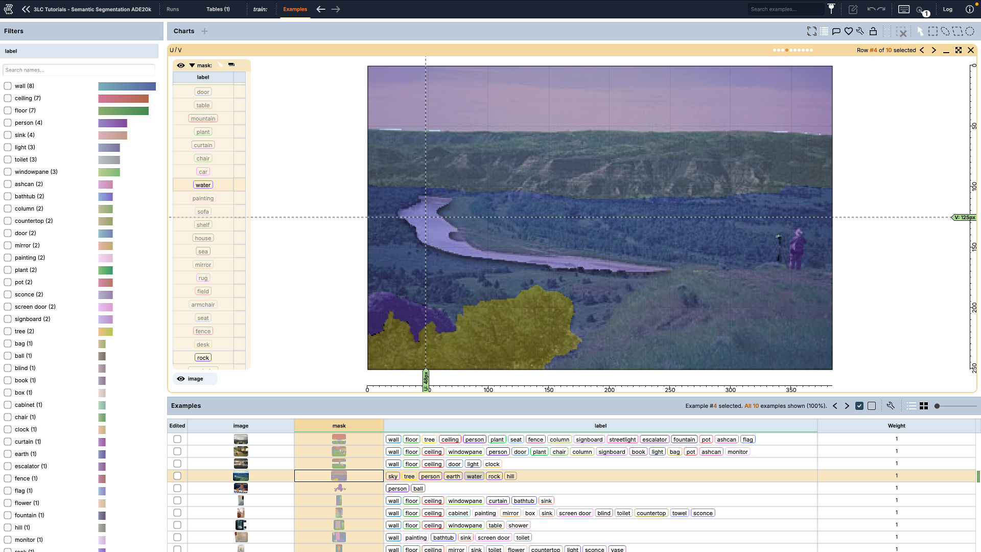
Image segmentation is a fundamental computer vision task that divides images into meaningful parts by assigning labels to individual pixels. This enables machines to understand the content and structure of images at a detailed level.

3LC supports two main types of segmentation. Semantic segmentation assigns class labels to pixels (e.g., all ‘car’ pixels get same label), focusing on what object types are present in the image and where. See Instance Segmentation for instance-level segmentation.

Creating a table

The front door for authoring a semantic-segmentation table is Table.from_semantic_segmentation(). Hand it the source images and their dense (H, W) integer label masks, declare the class universe, and it writes an image column plus an RLE-backed mask column:

import tlc

table = tlc.Table.from_semantic_segmentation(
    images=["img_0.png", "img_1.png"],   # PIL images, or path/URL strings
    masks=[mask_0, mask_1],              # (H, W) int arrays of class ids
    classes=["background", "car", "person"],
    background=0,
    project_name="Segmentation Project",
    dataset_name="train",
)

Each pixel in a mask holds a class id; every id must be declared in classes. The returned object is a plain Table — its “semseg-ness” lives in the mask column’s schema, not in a Python subtype. On read, the mask column yields SemanticSegmentation objects carrying the dense (H, W) label map.

Tip

images and masks don’t have to be materialized lists. They can be any indexable sequence — an object with __len__ and __getitem__ — so for large datasets you can pass a lazy sequence that loads and decodes each mask only when the writer reads it, instead of holding every mask in memory at once. This is the recommended pattern whenever the masks need per-item loading or preprocessing (e.g. decoding a PNG or remapping label ids); the Oxford Pets and Pascal VOC tutorials below both use it.

Background and void

Two class roles are handled specially, and you opt into them with the background and void arguments:

• background — the implicit fill. Its id is recorded in the column schema’s metadata (not the value map) and omitted from per-row storage at any id, then recovered as the fill on read. Background is not a class; it is rendered transparent in the Dashboard. Omit background entirely if your data has no background.

• void — the “don’t care” / ignore / boundary region (e.g. the 255 border in Pascal VOC). It stays a tagged class in the value map but is excluded from metrics downstream.

Metrics

Per-image segmentation metrics are built from a single primitive — a per-image C×C confusion matrix. semantic_segmentation_metrics() takes a predicted and a ground-truth label map plus the same classes / background / void vocabulary used above, and returns the per-image readouts — IoU, mean IoU, pixel accuracy, recall, Dice, and frequency-weighted IoU — alongside the confusion matrix itself. void pixels are excluded from every readout, and background is counted toward mean IoU when include_background is set.

Because each row carries its own confusion matrix, the cumulative, benchmark-correct headline mean IoU is obtained by summing the per-image matrices across rows and re-deriving from the total — not by averaging the per-image mean-IoU scalars. The training tutorials below show this metrics-collection path end to end.

Storage

Masks are stored compactly in a run-length-encoded (RLE) layout — one RLE per class actually present in the image, never an empty layer for an absent class. This supersedes the earlier PNG-file representation and is the format the Dashboard’s dedicated semantic-segmentation interface expects.

Lower-level schema

When you need finer control — e.g. authoring with a TableWriter or Table.from_dict() — declare the mask column directly with SemanticSegmentationRleSchema:

import tlc

writer = tlc.TableWriter(
    project_name="Segmentation Project",
    dataset_name="train",
    schema={
        "image": tlc.schemas.ImageSchema(),
        "mask": tlc.schemas.SemanticSegmentationRleSchema(
            classes=["background", "car", "person"],
            background=0,
        ),
    },
)

for img, mask in my_data:
    writer.add_row({"image": img, "mask": mask})

table = writer.finalize()

Note

A mask may be supplied in any of these forms — they all normalize to the same dense (H, W) label map: a 2-D numpy array of class ids, a single-channel PIL.Image, a path or URL string to a single-channel label-map image, or an explicit SemanticSegmentation. This holds for both Table.from_semantic_segmentation() and rows written through SemanticSegmentationRleSchema.

Deprecated: SemanticSegmentationSchema

The earlier SemanticSegmentationSchema, which stored masks as single-channel grayscale PNG files (one pixel value per class index), is deprecated and now emits a DeprecationWarning on use. It remains available for backwards compatibility, but new tables should use Table.from_semantic_segmentation() / SemanticSegmentationRleSchema instead.

Visualization and Editing

Create mask+image chart

Select the mask and image columns and click Create 2D chart in the chart area to create a mask+image chart. Click the triangle icon in the mask context menu to expand or collapse the list of segmentations. Selecting a segmentation on the chart highlights the corresponding entry in the mask list, and selecting an entry in the mask list selects it on the chart. When the list has more than 10 segmentations, a search box appears at the top so you can find one quickly. Segmentations that are not present on the displayed sample are grayed out and listed below the available ones.

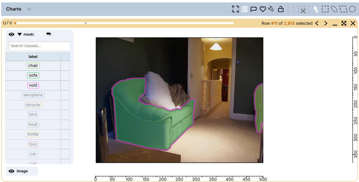
Semantic segmentation list vs BBs/instance segmentation list

• Semantic segmentation: the list shows all existing segmentation classes, with one entry per class.

• BBs/instance segmentation: the list shows all existing instances, with one entry per instance.

Edit a semantic segmentation mask

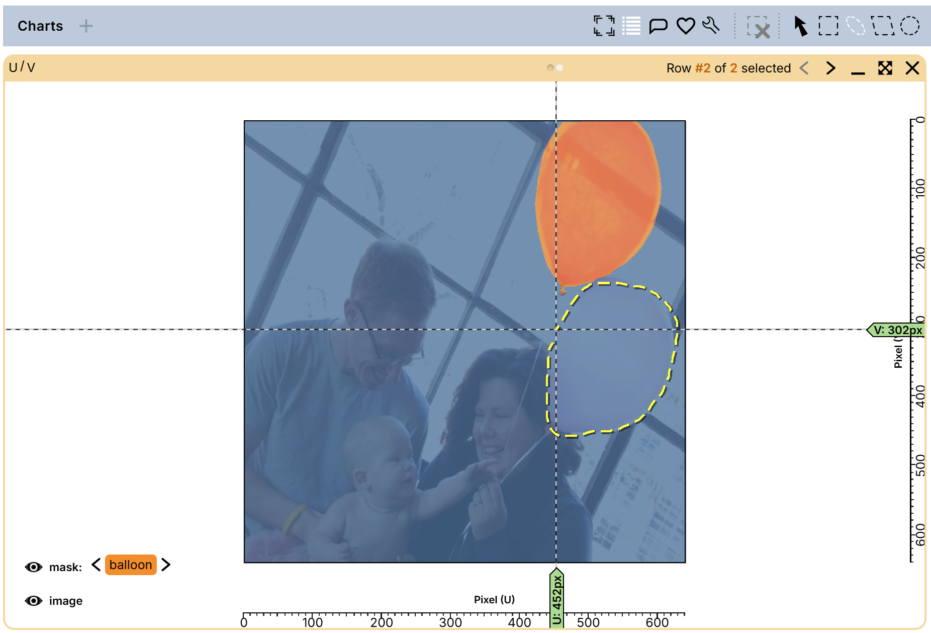
To edit a semantic mask, first select the segmentation you want to edit — either on the mask chart or in the expanded mask list. Then choose one of the selection tools on the chart toolbar to paint onto that segmentation.

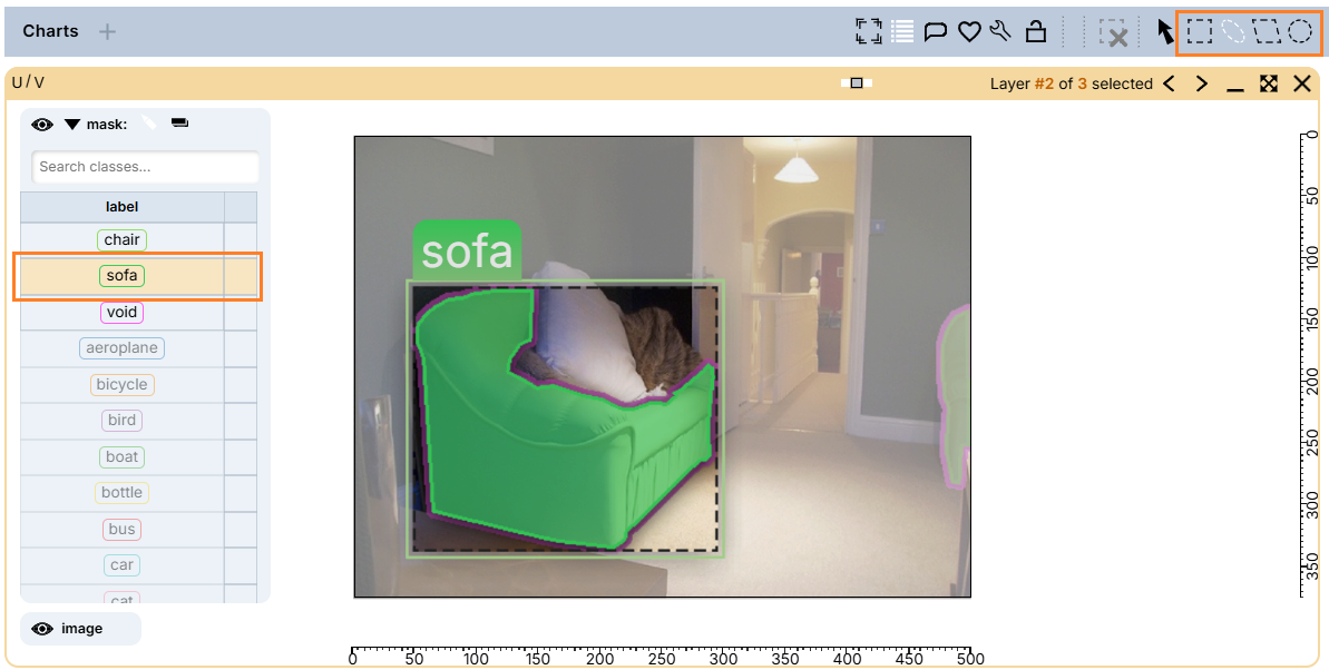
For example, the lasso tool lets you draw an outline directly on the mask chart. The other selection tools work the same way, so use whichever best suits the region you are editing. Any painted pixels that previously belonged to another segmentation are reassigned to the one you are painting.

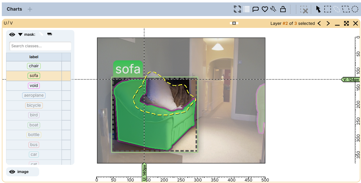
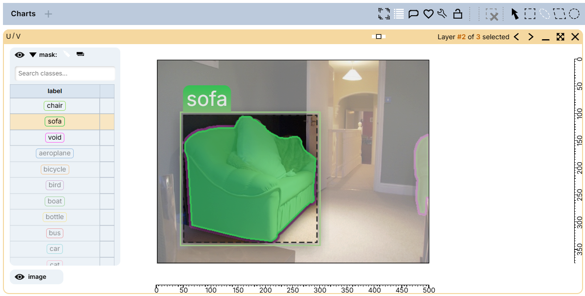
When you release the mouse button, the area inside the outline is filled with the color of the selected segmentation. Keep drawing to refine the same segmentation, or select a different segmentation first to edit another one.

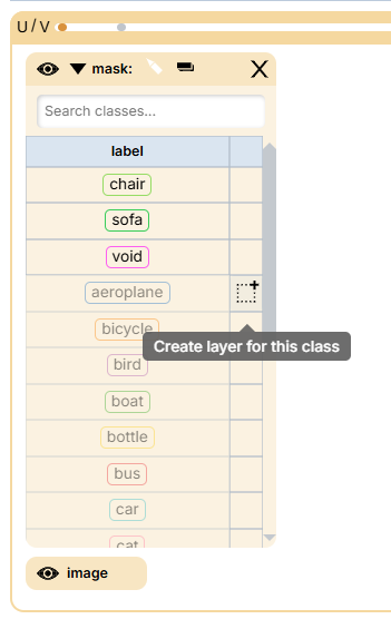
To edit a segmentation that is not currently present in a given sample, hover over that segmentation in the mask list — a Create a layer for this class icon appears — and click it. You can then paint on the segmentation as described above. Conversely, to delete an entire segmentation, hover over a segmentation that is present in the sample and click the trash-can icon that appears.

Accept predictions

You can convert a model’s predicted mask to a ground truth mask. To do this, first create an image + predicted mask chart, then RightClick on an empty area in the chart to bring up the context menu and click on Immediately accept predictions this row or press I to accept the current sample’s predicted mask as the ground truth. The ground truth mask will be updated to be the same as the predicted one.

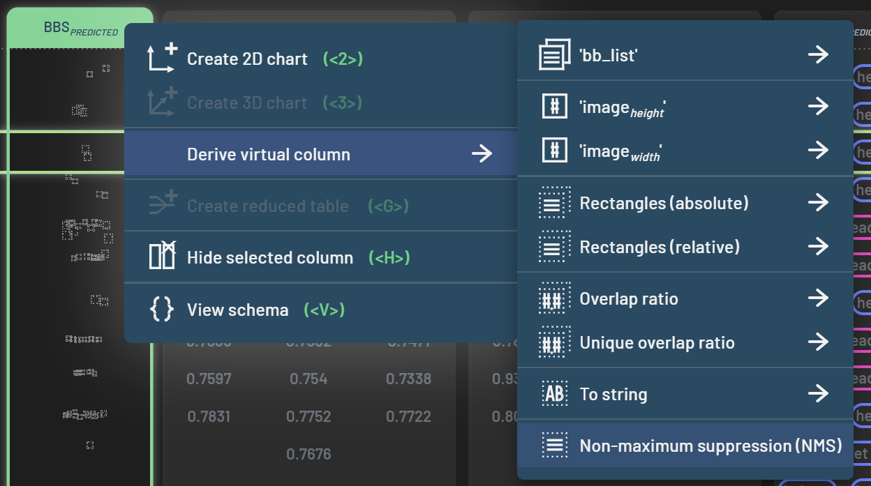
You can accept the predicted masks for all filtered-in samples at once by RightClicking the predicted_segmentation context menu and clicking Immediately accept all predictions or simply pressing B. Note that accepting semantic segmentation predictions will replace the entire existing ground truth segmentation mask with the predicted segmentations for a given sample.

Workflows for semantic segmentation

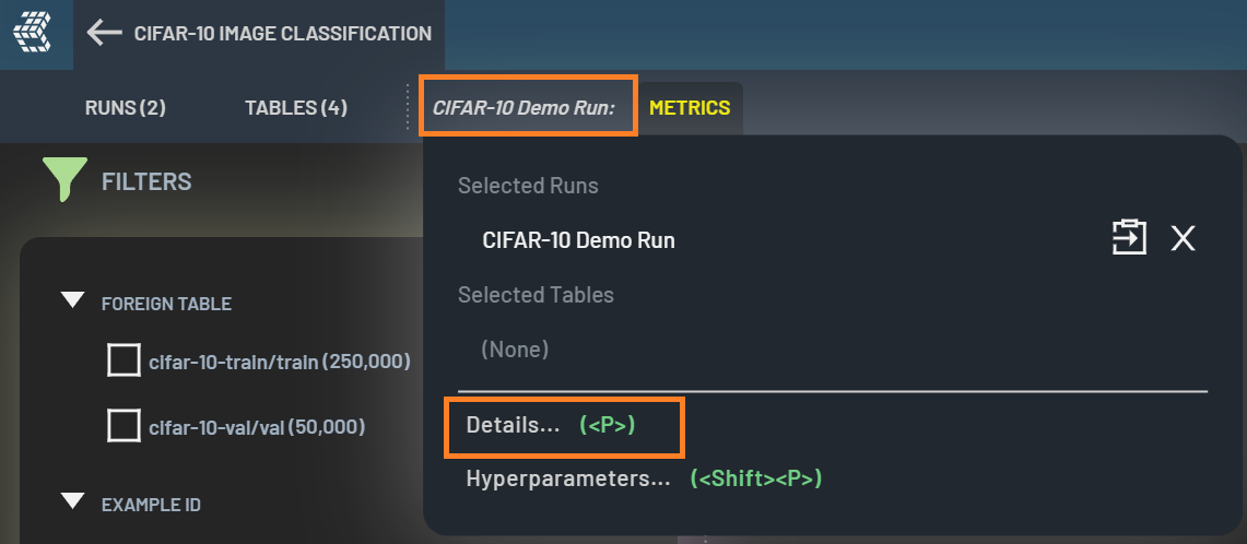
Some workflows are designed specifically for semantic segmentation. For instance, the Semantic segmentation confusion matrix workflow derives a confusion matrix for a semantic segmentation run. Select both ground truth mask and predicted_segmentation columns to get the workflow context menu.

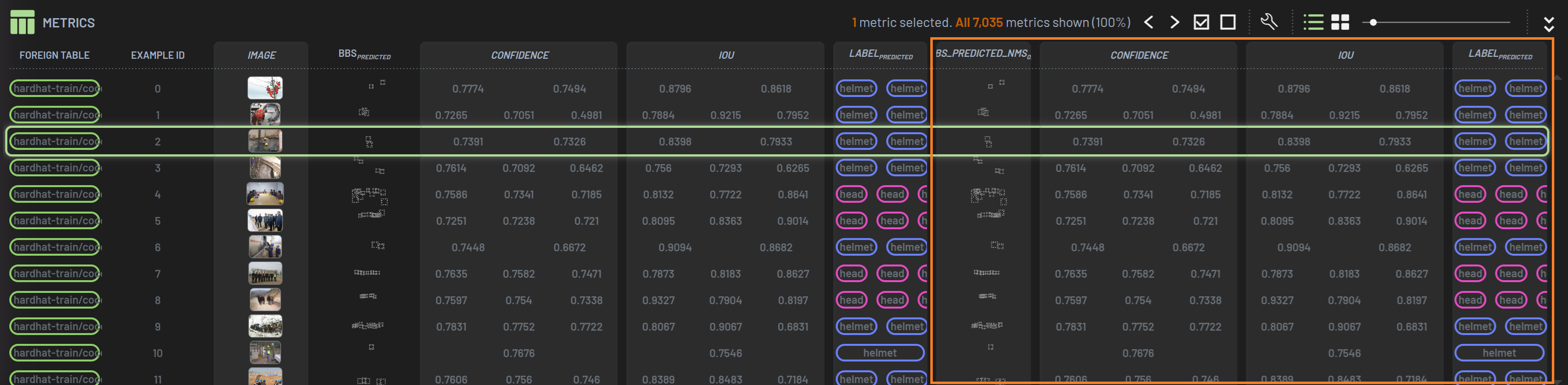
Launching this workflow creates a confusion matrix. It is similar to the instance confusion matrix, but it is computed over pixel pairs rather than instance pairs. Clicking a box in the confusion matrix filters to the samples that contain that confusion pair.

Tutorials

The following tutorials walk through creating semantic-segmentation tables and training models with metrics collection:

Tutorial	Task	Dataset	Description
create-ade20k-semseg-table.ipynb	Create table	ADE20K	Minimal ingest from paired images and label-map PNGs; id 0 (unlabeled) tagged as void
create-oxford-pets-semseg-table.ipynb	Create table	Oxford-IIIT Pet	Builds a semseg table from trimap masks (pet / background / border) with an implicit background and a tagged void class
create-pascal-voc-semseg-table.ipynb	Create table	Pascal VOC	Builds a 21-class semseg table directly from VOC’s paletted PNGs, with background in metadata and the 255 boundary as void
pytorch-oxford-pets-unet-training.ipynb	Training	Oxford-IIIT Pet	Trains a U-Net and collects per-sample segmentation metrics
huggingface-pascal-voc-mask2former-finetuning.ipynb	Training	Pascal VOC	Fine-tunes a Mask2Former model and collects metrics
huggingface-sugarbeets-segformer-training.ipynb	Training	Sugarbeets	Fine-tunes a SegFormer semantic-segmentation model
lightning-balloons-segformer-training.ipynb	Training	Balloons	Fine-tunes a SegFormer model with PyTorch Lightning (uses the legacy PNG-mask format)