Create a Semantic Segmentation Table from Oxford-IIIT Pets¶

Ingest the Oxford-IIIT Pets dataset into 3LC tables for semantic segmentation. Each image has a trimap giving three classes — pet, background, and border — stored as run-length-encoded layers.

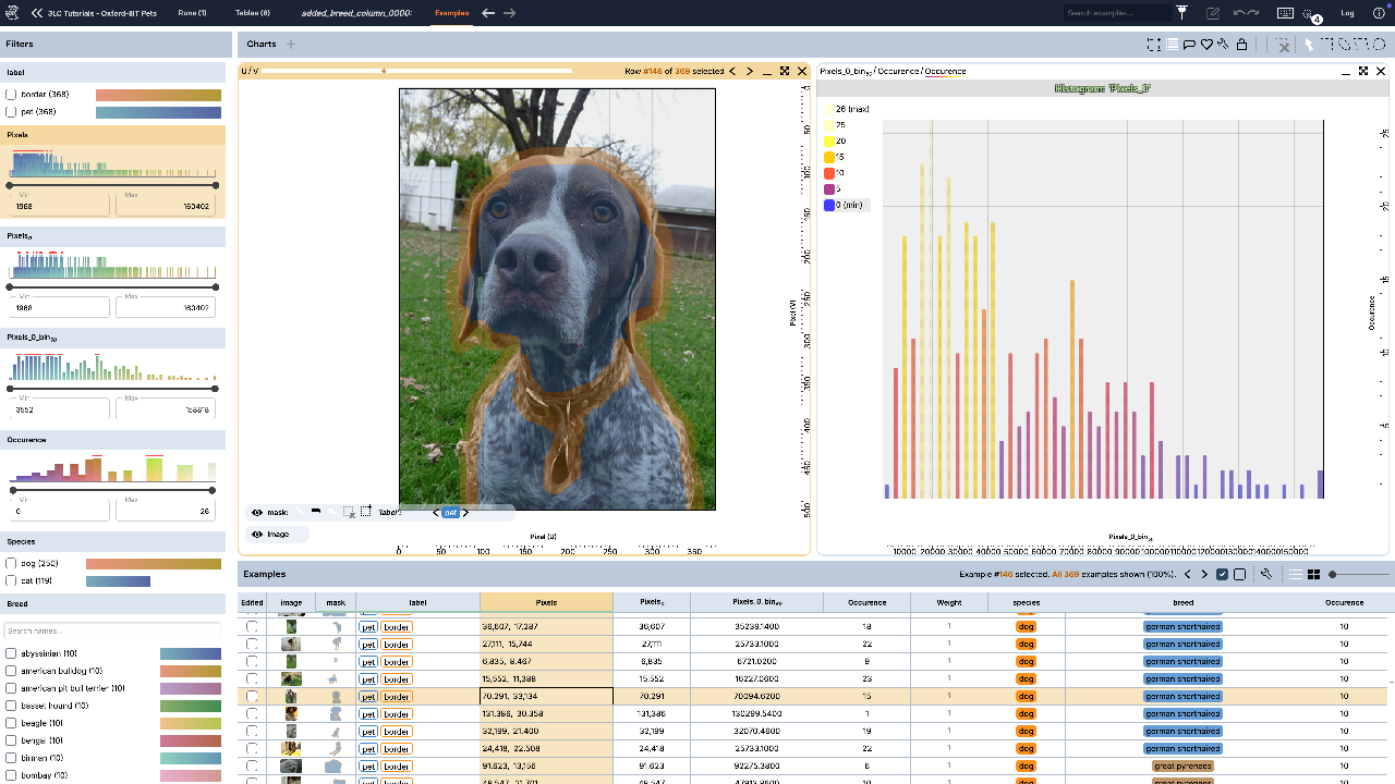
Semantic segmentation assigns every pixel a class label, producing a dense (H, W) map that exhaustively partitions the image. We ingest Oxford-IIIT Pets through the documented front door Table.from_semantic_segmentation, which takes the images and the raw integer masks directly and writes an image column plus an RLE-backed mask column. background is implicit — omitted from both per-row storage and the value map (its id rides in the column schema’s metadata) and recovered on read — keeping storage compact. We then attach the per-image species and breed labels with Table.add_column.

This is the ingest half of a pair: the companion notebook pytorch-oxford-pets-unet-training trains a UNet on the tables created here and collects per-sample metrics back into 3LC.

Project setup¶

[ ]:

# Parameters
PROJECT_NAME = "3LC Tutorials - Oxford-IIIT Pets"
DATASET_NAME = "oxford-iiit-pets"
TABLE_NAME = "train"
VAL_TABLE_NAME = "val"
DOWNLOAD_PATH = "../../transient_data"  # dataset root; point at an existing copy to skip the download
VAL_FRACTION = 0.1  # held-out val slice of the official trainval split (stratified by breed); test stays out
N_TRAIN = None  # cap the train rows for a quick run; None keeps the whole train split
N_VAL = None  # cap the val rows for a quick run; None keeps the whole val split
SEED = 42
INSTALL_DEPENDENCIES = True

Install dependencies¶

[ ]:

if INSTALL_DEPENDENCIES:
    %pip install -q 3lc torchvision matplotlib

Imports¶

[ ]:

import random
from collections.abc import Sequence
from pathlib import Path

import numpy as np
import tlc
from PIL import Image
from torchvision.datasets import OxfordIIITPet

Download the dataset¶

torchvision handles the download — one call fetches the whole dataset, including both the trainval and test annotation lists. We only need it to fetch the files; afterwards we read the images and trimaps straight from disk so the Table references the original image files by URL (rather than re-encoding them).

The download only runs when the data is missing: if DOWNLOAD_PATH/oxford-iiit-pet/ already exists, torchvision uses it as-is and never writes (so a pre-seeded read-only cache is safe). To reuse an existing copy, point DOWNLOAD_PATH at its parent — e.g. DOWNLOAD_PATH = "~/data" when the dataset lives at ~/data/oxford-iiit-pet.

[ ]:

download_root = Path(DOWNLOAD_PATH).expanduser()
data_root = download_root / "oxford-iiit-pet"
# Only download when missing — torchvision needs both images/ and annotations/ to consider it present.
have_data = (data_root / "images").is_dir() and (data_root / "annotations").is_dir()
print(
    f"Dataset cache {'HIT' if have_data else 'MISS'} at {data_root.resolve()} "
    f"({'using existing data' if have_data else 'downloading'})"
)
OxfordIIITPet(root=download_root, split="trainval", target_types="segmentation", download=not have_data)
print("Dataset at", data_root.resolve())

Define the class universe¶

The trimap stores three pixel values, and we keep them exactly as they appear in the source masks — 1 = pet, 2 = background, 3 = border — no remapping. Two classes get special roles, declared via the background / void arguments to the front door:

background (id 2) — not a class in the value map. Its id is recorded in the column schema’s metadata, and the background is omitted from per-row storage (the implicit fill) and recovered on read. Rendered transparent in the Dashboard.
border (id 3) — tagged void (a “don’t care” ring around each pet), so it can be excluded from the loss and from metrics like mean IoU.

[ ]:

# The trimap PNG already holds the class ids: 1 = pet, 2 = background, 3 = border. We store them as-is.
SEGMENTATION_CLASSES = {1: "pet", 2: "background", 3: "border"}
BACKGROUND_ID = 2
VOID_ID = 3
SPECIES_CLASSES = ["cat", "dog"]

Parse the annotations and split¶

Oxford-IIIT Pets ships an official partition: trainval.txt (the train pool) and test.txt (the held-out benchmark set). There is no canonical sub-split of trainval, so we make our own — parse trainval and carve off a VAL_FRACTION validation slice, stratified by breed so all 37 breeds are represented in both tables. test.txt is deliberately left untouched as the final benchmark. Each list line is IMAGE CLASS-ID SPECIES BREED-ID, giving breed (37 classes) and species (cat/dog) and locating the trimap.

[ ]:

def parse_annotations(root: Path, split: str) -> list[dict]:
    # Parse annotations/<split>.txt (split is "trainval" or "test") into per-sample dicts.
    samples = []
    for line in (root / "annotations" / f"{split}.txt").read_text().splitlines():
        if line.startswith("#") or not line.strip():
            continue
        name, class_id, species, _breed_id = line.split()
        image_path = root / "images" / f"{name}.jpg"
        trimap_path = root / "annotations" / "trimaps" / f"{name}.png"
        if not image_path.exists() or not trimap_path.exists():
            continue
        samples.append(
            {
                "name": name,
                "image_path": image_path.resolve(),
                "trimap_path": trimap_path.resolve(),
                "breed": int(class_id) - 1,  # 0-based
                "species": int(species) - 1,  # 0: cat, 1: dog
            }
        )
    return samples


def breed_names(samples: list[dict]) -> list[str]:
    # Derive 0-indexed breed names from the image file names.
    names: dict[int, str] = {}
    for s in samples:
        names[s["breed"]] = s["name"].rsplit("_", 1)[0].replace("_", " ").lower()
    return [names[i] for i in range(max(names) + 1)]


def stratified_split(samples: list[dict], val_fraction: float, seed: int) -> tuple[list[dict], list[dict]]:
    # Deterministic per-breed split so train and val share the same 37-breed distribution.
    by_breed: dict[int, list[dict]] = {}
    for s in samples:
        by_breed.setdefault(s["breed"], []).append(s)
    rng = random.Random(seed)
    train, val = [], []
    for breed in sorted(by_breed):
        items = by_breed[breed]
        rng.shuffle(items)
        n_val = max(1, round(len(items) * val_fraction))  # at least one val image per breed
        val.extend(items[:n_val])
        train.extend(items[n_val:])
    return train, val


# Split the official trainval pool into train/val (stratified by breed); test.txt stays held out.
trainval_samples = parse_annotations(data_root, "trainval")
train_samples, val_samples = stratified_split(trainval_samples, VAL_FRACTION, SEED)
breeds = breed_names(trainval_samples)
print(
    f"Split {len(trainval_samples)} trainval images -> {len(train_samples)} train + {len(val_samples)} val "
    f"across {len(breeds)} breeds (test.txt held out)"
)

Decode trimaps into dense masks¶

The front door takes the masks as a sequence of dense (H, W) integer arrays. TrimapMasks decodes each PNG on indexed access — the pixel values are already the class ids — so we never hold every mask in memory at once.

[ ]:

class TrimapMasks(Sequence):
    def __init__(self, trimap_paths: list[Path]) -> None:
        self._trimap_paths = trimap_paths

    def __len__(self) -> int:
        return len(self._trimap_paths)

    def __getitem__(self, index: int) -> np.ndarray:
        # The trimap PNG's pixel values are the class ids (1 = pet, 2 = background, 3 = border).
        return np.asarray(Image.open(self._trimap_paths[index]), dtype=np.int32)

Write the tables¶

Table.from_semantic_segmentation writes the image and mask columns in one call, recording the background id in the schema metadata and tagging the void class. We then attach the per-image species and breed labels with Table.add_column (each returns a new revision of the table). The train and val tables are the breed-stratified split of trainval from the previous cell; by default all rows are used, with N_TRAIN / N_VAL capping each for a quick run.

The front door covers the image + mask case; add_column is the general way to attach extra per-row columns. For very large datasets you may prefer to author all columns in a single TableWriter pass.

[ ]:

def write_table(rows: list[dict], table_name: str) -> tlc.Table:
    table = tlc.Table.from_semantic_segmentation(
        images=[s["image_path"] for s in rows],
        masks=TrimapMasks([s["trimap_path"] for s in rows]),
        classes=SEGMENTATION_CLASSES,
        background=BACKGROUND_ID,
        void=VOID_ID,
        project_name=PROJECT_NAME,
        dataset_name=DATASET_NAME,
        table_name=table_name,
        if_exists="overwrite",
    )
    table = table.add_column(
        "species", [s["species"] for s in rows], schema=tlc.schemas.CategoricalLabelSchema(SPECIES_CLASSES)
    )
    table = table.add_column("breed", [s["breed"] for s in rows], schema=tlc.schemas.CategoricalLabelSchema(breeds))
    print(f"Wrote {table_name}: {len(table)} rows -> {table.url}")
    return table


def select(rows: list[dict], n: int | None) -> list[dict]:
    # None -> use every row; otherwise take a deterministic random subset of n rows.
    if n is None:
        return rows
    return random.Random(SEED).sample(rows, min(n, len(rows)))


train_table = write_table(select(train_samples, N_TRAIN), TABLE_NAME)
val_table = write_table(select(val_samples, N_VAL), VAL_TABLE_NAME)

Inspect a sample¶

Reading a row back hands you the dense mask plus the categorical labels. We overlay the mask on the image to sanity-check the alignment.

[ ]:

import matplotlib.pyplot as plt

sample = train_table[0]
seg = sample["mask"]
print(f"Classes present: {seg.present_class_ids.tolist()}")

image = sample["image"]
mask = seg.mask  # dense (H, W) label map

fig, axes = plt.subplots(1, 2, figsize=(9, 4))
axes[0].imshow(image)
axes[0].set_title(f"{breeds[sample['breed']]} ({SPECIES_CLASSES[sample['species']]})")
axes[1].imshow(image)
axes[1].imshow(mask, alpha=0.5, cmap="viridis", interpolation="nearest")
axes[1].set_title("background / pet / border")
for ax in axes:
    ax.axis("off")
plt.tight_layout()
plt.show()

Next steps¶

The train and val tables are now in your 3LC project — open the project in the 3LC Dashboard to browse the images and their segmentations.

Continue with pytorch-oxford-pets-unet-training to train a UNet on these tables and collect per-sample predictions, IoU, and embeddings back into a 3LC Run.